

How Successful Is Your Region at Retaining Its Native Residents?
This District Data Brief analyzes how well regions in the Fourth District and across the United States retain their native residents and whether their retention rates are associated with population growth.
The views authors express in District Data Briefs are theirs and not necessarily those of the Federal Reserve Bank of Cleveland or the Board of Governors of the Federal Reserve System. The series editor is Harrison Markel.
Introduction
How can our region stop people from moving away? This question regularly arises in conversations among local leaders across the country. Before asking this question, it would be helpful to know whether one’s region is already successful at keeping its native residents. Using long histories of individuals’ locations drawn from the Federal Reserve Bank of New York/Equifax Consumer Credit Panel, we can begin to answer this question by measuring retention. We find that Fourth District metros with populations of greater than 1 million are better than average at retaining their natives but that retaining a high share of natives is not associated with strong regional population growth.
Data and Definitions
The estimates of individuals’ long-run patterns of migration are created with a random, anonymous sample drawn from credit histories maintained by Equifax, known as the Federal Reserve Bank of New York/Equifax Consumer Credit Panel (CCP). Almost nine of 10 adults in the United States have accounts with creditors (for example, mortgages, student loans, auto loans, and credit cards), and these lenders report billing addresses to the credit bureaus each month. The CCP data include the county that contains the borrower’s billing address, and this enables us to observe each quarter whether an individual is living in their home region or another region. When borrowers first apply for credit, we designate them as a native of the region in which they are living.1 Because the CCP begins in 1999, we must limit the analysis to people born in 1981 or later, as credit histories do not start until age 18 (typically between 18 and 23) and we need to observe people when their credit history begins to accurately place them in their home region.
Some of the results presented below are disaggregated by credit score. The score available in the CCP is the Equifax Risk Score. Like other credit scores, it uses information in borrowers’ credit records to predict the probability of their becoming delinquent on debts.
In this District Data Brief, the term “metro” refers to a Core-Based Statistical Area (CBSA) as defined by the Office of Management and Budget (OMB). The US Department of Agriculture groups rural counties into regions called “commuting zones” (CZs) based on how frequently people drive between the counties for work. We use the CZ definitions for all nonmetro counties so that we can include all counties in our calculations. We define “large metros” as those with populations of greater than 1 million for graphs of the top-10 and bottom-10 metros. To better illustrate certain relationships, the samples in scatterplots include all regions with populations of greater than 500,000.
Retention of Natives
We calculate our measure of native retention by dividing the total number of quarters that native individuals are living in their home region by the total number of quarters we can observe for every person native to that region in the CCP data. Figure 1 shows this measure for the top 10 and bottom 10 large metros nationally in terms of native retention. Among the top 10 large metros, some, including Houston, Dallas, and Phoenix, are fast-growing. Meanwhile, others, such as New York, Los Angeles, Chicago, and Memphis, are slow-growing. The bottom 10 large metros include some that are seeing rapid growth, such as Austin, Orlando, and Raleigh. They also include Honolulu and San Jose, which have some of the highest costs of living in the country.

Sources: Federal Reserve Bank of New York/Equifax Consumer Credit Panel and authors’ calculations. “High-score” estimates limit the sample to individuals with Equifax Risk Scores in the top third of the distribution.
It is reasonable to ask whether remaining in one’s home region is voluntary. People in some regions might stay because they do not have skills that are in demand anywhere else. Additionally, they may lack the savings or credit necessary to move. To understand whether a region is retaining people that could leave if they wanted to, we can focus on individuals with higher Equifax Risk Scores. These are people who have been able to consistently repay their lenders and could borrow to pay for moving expenses. When we calculate the native retention measure for only people with Equifax Risk Scores in the top third of the score distribution (indicated with green bars in Figures 1 and 2), we see that the pattern for these individuals is similar to that for the full sample, but with some notable differences.
Retention of high-score individuals is usually lower than overall retention. This is intuitive if we recall that higher credit scores are positively related to earning power and earning power generally increases with education. We know from Census data that people who go further in postsecondary education are more likely to search for jobs nationally and move. There are a few exceptions to the pattern of lower retention of high-score individuals, including in San Jose, Honolulu, Los Angeles, and New York. In these cases, very high costs of living may motivate households with weaker finances to move away, making overall retention similar to or below the retention rate of high-score individuals.
If we take an average over all the periods we can observe for all the people in the sample, we find they are retained (that is, living in their home metro) 78 percent of the time. However, when we calculate this same average for every region, we find a divide between regions with large and small populations. The average retention rate is 72 percent for regions with populations of less than 1 million and 83 percent for those with more than 1 million.
The positive relationship between population size and native retention can be seen in the Fourth District as well. The four most populous metros of the Fourth District have more diversified economies, so natives are more likely to find a good match with an employer and be able to stay near their family and friends. As shown in Figure 2, native retention rates in Cleveland (80.1 percent), Columbus (82.1 percent), Pittsburgh (83 percent), and Cincinnati (83 percent) are all above the national average. The rates of the other Fourth District metros are 1 to 4 percentage points below the national average.
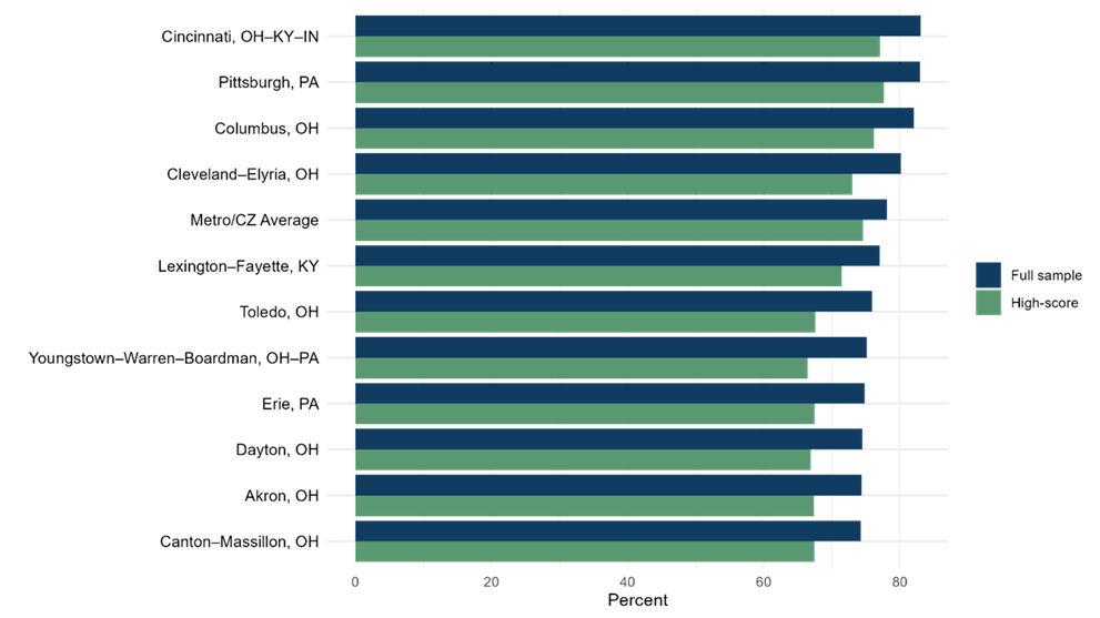
Sources: Federal Reserve Bank of New York/Equifax Consumer Credit Panel and authors’ calculations. “High-score” estimates limit the sample to individuals with Equifax Risk Scores in the top third of the distribution.
Figure 3 plots population growth against native retention for all US metros with populations of over 500,000. It includes a population-weighted line of best fit to summarize the relationship between the two measures. Arithmetically, every person retained makes population growth higher or population loss smaller. However, the fastest-growing places are not those that are best at retaining people who were born there. Many places that are barely growing retain a higher portion of their natives. Retaining a greater-than-average share of natives is not sufficient to guarantee higher-than-average population growth.
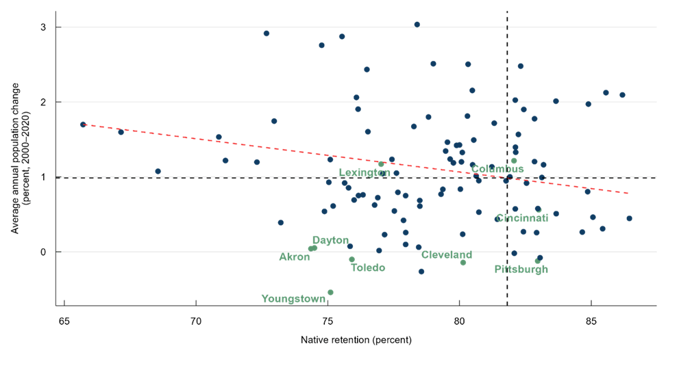
Sources: Census Bureau, Federal Reserve Bank of New York/Equifax Consumer Credit Panel, and authors’ calculations. The Fourth District metros are indicated by green markers and labels.
Conclusion
In this analysis, we learned that variation in native retention rates is quite narrow across the United States. Most regions retain their natives for between 75 and 85 percent of the time that we can observe them, with the national average at 78 percent. More populous regions generally have higher retention rates. Returning to the question of whether our regions are already successful at retaining natives, we have learned that, among Fourth District metros, Cincinnati, Columbus, Pittsburgh, and Cleveland compare favorably to the national average on this dimension, with retention rates of 80 to 83 percent. Rather than guaranteeing regions grow their populations, native retention appears to have, if anything, a negative relationship to population growth. This suggests regions that are growing must be doing so by attracting people from outside the region to move in and stay. We will examine this further in an upcoming District Data Brief.
Footnotes
- Some students might use a college dormitory address in their first application for credit. If they are attending school out of town, they may be labeled natives of the wrong region. This could bias the estimates of retention, especially for college towns, because these students are likely to return home or move on after graduation. To account for this, we estimate the relationship between regions’ student populations and their retention. We then adjust each region’s retention estimate to remove the effect of students. Return to 1
Appendix
Table A1. Share of Natives’ Quarters Spent in Their Original Region (Populations >500,000)
| Metro area | Native retention rate | Metro area | Native retention rate | ||
| Full sample | High-score | Full sample | High-score | ||
| New York–Newark–Jersey City, NY–NJ–PA | 86.45 | 86.54 | Washington–Arlington–Alexandria, DC–VA–MD–WV | 79.47 | 76.33 |
| Houston–The Woodlands–Sugar Land, TX | 86.18 | 80.63 | Chattanooga, TN–GA | 79.37 | 72.55 |
| McAllen–Edinburg–Mission, TX | 85.56 | 79.86 | San Diego–Carlsbad, CA | 79.30 | 79.10 |
| Los Angeles–Long Beach–Anaheim, CA | 85.43 | 85.74 | Boise City, ID | 79.01 | 77.08 |
| Philadelphia–Camden–Wilmington, PA–NJ–DE–MD | 85.06 | 81.11 | Ogden–Clearfield, UT | 78.82 | 79.04 |
| Dallas–Fort Worth–Arlington, TX | 84.89 | 80.30 | New Orleans–Metairie, LA | 78.55 | 74.86 |
| Louisville/Jefferson County, KY–IN | 84.86 | 80.51 | Wichita, KS | 78.49 | 74.18 |
| Chicago–Naperville–Elgin, IL–IN–WI | 84.66 | 82.15 | San Francisco–Oakland–Hayward, CA | 78.49 | 79.81 |
| Memphis, TN–MS–AR | 83.67 | 76.02 | Scranton––Wilkes–Barre––Hazleton, PA | 78.45 | 71.93 |
| Phoenix–Mesa–Scottsdale, AZ | 83.66 | 80.69 | Austin–Round Rock, TX | 78.39 | 73.24 |
| Fresno, CA | 83.19 | 80.55 | Des Moines–West Des Moines, IA | 78.27 | 73.57 |
| Minneapolis–St. Paul–Bloomington, MN–WI | 83.13 | 81.51 | Hartford–West Hartford–East Hartford, CT | 77.96 | 73.97 |
| Detroit–Warren–Dearborn, MI | 83.06 | 79.29 | Rochester, NY | 77.96 | 71.36 |
| Cincinnati, OH–KY–IN | 83.01 | 77.09 | Grand Rapids–Wyoming, MI | 77.95 | 76.58 |
| Birmingham–Hoover, AL | 82.97 | 77.81 | Albany–Schenectady–Troy, NY | 77.87 | 73.37 |
| Pittsburgh, PA | 82.97 | 77.65 | Lancaster, PA | 77.66 | 75.35 |
| St. Louis, MO–IL | 82.93 | 78.70 | Tucson, AZ | 77.61 | 70.71 |
| Atlanta–Sandy Springs–Roswell, GA | 82.85 | 78.63 | Oxnard–Thousand Oaks–Ventura, CA | 77.53 | 76.77 |
| Indianapolis–Carmel–Anderson, IN | 82.85 | 77.16 | Columbia, SC | 77.43 | 69.84 |
| Baton Rouge, LA | 82.54 | 75.01 | New Haven–Milford, CT | 77.16 | 71.48 |
| Nashville–Davidson––Murfreesboro––Franklin, TN | 82.44 | 79.28 | Modesto, CA | 77.09 | 75.27 |
| Providence–Warwick, RI–MA | 82.43 | 78.41 | Lexington–Fayette, KY | 77.02 | 71.48 |
| Las Vegas–Henderson–Paradise, NV | 82.32 | 80.83 | Springfield, MA | 76.95 | 69.88 |
| Bakersfield, CA | 82.23 | 80.67 | Urban Honolulu, HI | 76.90 | 79.10 |
| Oklahoma City, OK | 82.13 | 77.76 | Worcester, MA–CT | 76.78 | 72.20 |
| Seattle–Tacoma–Bellevue, WA | 82.12 | 82.15 | Stockton–Lodi, CA | 76.52 | 73.89 |
| Boston–Cambridge–Newton, MA–NH | 82.12 | 80.16 | Orlando–Kissimmee–Sanford, FL | 76.48 | 74.15 |
| San Antonio–New Braunfels, TX | 82.12 | 74.36 | Harrisburg–Carlisle, PA | 76.34 | 72.29 |
| Buffalo–Cheektowaga–Niagara Falls, NY | 82.08 | 76.43 | Allentown–Bethlehem–Easton, PA–NJ | 76.16 | 70.71 |
| Columbus, OH | 82.07 | 76.19 | Charleston–North Charleston, SC | 76.15 | 66.55 |
| Miami–Fort Lauderdale–West Palm Beach, FL | 81.91 | 78.78 | Lakeland–Winter Haven, FL | 76.09 | 70.50 |
| Kansas City, MO–KS | 81.77 | 77.45 | San Jose–Sunnyvale–Santa Clara, CA | 76.00 | 75.68 |
| Jackson, MS | 81.43 | 73.87 | Toledo, OH | 75.91 | 67.62 |
| Riverside–San Bernardino–Ontario, CA | 81.32 | 80.08 | Syracuse, NY | 75.85 | 69.16 |
| Albuquerque, NM | 81.23 | 77.75 | Winston–Salem, NC | 75.79 | 68.36 |
| Baltimore–Columbia–Towson, MD | 80.74 | 75.60 | Greensboro–High Point, NC | 75.64 | 69.61 |
| Knoxville, TN | 80.73 | 75.01 | Raleigh, NC | 75.54 | 71.85 |
| Little Rock–North Little Rock–Conway, AR | 80.63 | 77.26 | Portland–South Portland, ME | 75.20 | 72.00 |
| Denver–Aurora–Lakewood, CO | 80.54 | 78.58 | Youngstown–Warren–Boardman, OH–PA | 75.10 | 66.44 |
| Omaha–Council Bluffs, NE–IA | 80.50 | 76.64 | Spokane–Spokane Valley, WA | 75.09 | 72.09 |
| Charlotte–Concord–Gastonia, NC–SC | 80.49 | 74.96 | Augusta–Richmond County, GA–SC | 75.04 | 66.00 |
| Fayetteville–Springdale–Rogers, AR–MO | 80.33 | 75.75 | Virginia Beach–Norfolk–Newport News, VA–NC | 74.87 | 69.86 |
| Jacksonville, FL | 80.30 | 75.84 | Cape Coral–Fort Myers, FL | 74.77 | 71.28 |
| Cleveland–Elyria, OH | 80.14 | 73.06 | Dayton, OH | 74.49 | 66.91 |
| Milwaukee–Waukesha–West Allis, WI | 80.12 | 75.36 | Akron, OH | 74.36 | 67.39 |
| Portland–Vancouver–Hillsboro, OR–WA | 80.11 | 77.73 | Bridgeport–Stamford–Norwalk, CT | 73.22 | 69.75 |
| El Paso, TX | 80.07 | 74.72 | North Port–Sarasota–Bradenton, FL | 72.96 | 68.86 |
| Tulsa, OK | 80.03 | 75.67 | Provo–Orem, UT | 72.67 | 72.96 |
| Sacramento––Roseville––Arden–Arcade, CA | 80.00 | 79.18 | Madison, WI | 72.31 | 69.93 |
| Tampa–St. Petersburg–Clearwater, FL | 79.89 | 76.18 | Palm Bay–Melbourne–Titusville, FL | 71.12 | 66.15 |
| Richmond, VA | 79.77 | 74.60 | Deltona–Daytona Beach–Ormond Beach, FL | 70.86 | 65.44 |
| Greenville–Anderson–Mauldin, SC | 79.64 | 70.35 | Durham–Chapel Hill, NC | 67.15 | 60.30 |
| Salt Lake City, UT | 79.54 | 77.76 | Colorado Springs, CO | 65.71 | 60.78 |
Sources: Federal Reserve Bank of New York/Equifax Consumer Credit Panel and authors' calculations. “High-score” estimates limit the sample to individuals with Equifax Risk Scores in the top third of the distribution.
Table A2. Share of Natives’ Quarters Spent in Their Original Region (Population-Weighted Average, Populations ≤500,000)
| Area | Native retention rate | Area | Native retention rate | ||
| Full sample | High-score | Full sample | High-score | ||
| Small metro and rural – Hawaii | 77.19 | 74.72 | Small metro and rural – North Carolina | 69.56 | 63.81 |
| Small metro and rural – Louisiana | 76.07 | 70.70 | Small metro and rural – Connecticut | 68.95 | 64.75 |
| Small metro and rural – Delaware | 75.71 | 71.75 | Small metro and rural – Ohio | 68.77 | 63.54 |
| Small metro and rural – West Virginia | 74.51 | 66.50 | Small metro and rural – New York | 68.56 | 63.46 |
| Small metro and rural – Alabama | 74.31 | 66.84 | Small metro and rural – New Hampshire | 68.47 | 63.29 |
| Small metro and rural – Kentucky | 73.98 | 68.05 | Small metro and rural – Florida | 68.40 | 64.21 |
| Small metro and rural – New Jersey | 73.15 | 69.04 | Small metro and rural – Washington | 68.18 | 65.54 |
| Small metro and rural – Tennessee | 73.05 | 68.83 | Small metro and rural – Oregon | 67.64 | 64.21 |
| Small metro and rural – Maryland | 72.71 | 68.30 | Small metro and rural – Missouri | 67.61 | 63.10 |
| Small metro and rural – California | 72.53 | 71.31 | Small metro and rural – Michigan | 67.10 | 63.06 |
| Small metro and rural – Pennsylvania | 71.59 | 66.94 | Small metro and rural – Wisconsin | 66.49 | 63.15 |
| Small metro and rural – Mississippi | 71.53 | 65.02 | Small metro and rural – Oklahoma | 66.42 | 61.96 |
| Small metro and rural – Massachusetts | 71.47 | 66.86 | Small metro and rural – Arizona | 65.14 | 61.97 |
| Small metro and rural – South Carolina | 71.43 | 64.00 | Small metro and rural – North Dakota | 65.11 | 62.24 |
| Small metro and rural – Nevada | 71.17 | 71.01 | Small metro and rural – Utah | 64.57 | 64.43 |
| Small metro and rural – Georgia | 71.05 | 64.60 | Small metro and rural – Wyoming | 64.13 | 61.27 |
| Small metro and rural – Arkansas | 70.88 | 66.71 | Small metro and rural – Montana | 64.08 | 60.70 |
| Small metro and rural – Maine | 70.86 | 65.01 | Small metro and rural – Idaho | 63.91 | 61.26 |
| Small metro and rural – Virginia | 70.57 | 63.90 | Small metro and rural – South Dakota | 63.89 | 59.25 |
| Small metro and rural – Vermont | 70.48 | 65.74 | Small metro and rural – Nebraska | 63.75 | 58.83 |
| Small metro and rural – Illinois | 70.33 | 64.89 | Small metro and rural – Colorado | 63.16 | 61.34 |
| Small metro and rural – Indiana | 70.17 | 65.20 | Small metro and rural – Minnesota | 63.06 | 59.91 |
| Small metro and rural – Alaska | 70.11 | 70.20 | Small metro and rural – Iowa | 62.74 | 57.30 |
| Small metro and rural – Texas | 69.98 | 62.65 | Small metro and rural – Kansas | 61.33 | 57.81 |
| Small metro and rural – New Mexico | 69.85 | 62.71 | |||
Sources: Federal Reserve Bank of New York/Equifax Consumer Credit Panel and authors’ calculations. “High-score” estimates limit the sample to individuals with Equifax Risk Scores in the top third of the distribution.
Suggested Citation
Whitaker, Stephan D., and Brett Huettner. 2024. “How Successful Is Your Region at Retaining Its Native Residents?” Federal Reserve Bank of Cleveland, Cleveland Fed District Data Brief. https://doi.org/10.26509/frbc-ddb-20241024
This work by Federal Reserve Bank of Cleveland is licensed under Creative Commons Attribution-NonCommercial 4.0 International


- Share