

Boomerang Migration: Which Regions Have the Most, and Can It Make a Difference?
This District Data Brief analyzes how well regions in the Fourth District and across the United States draw back native residents who previously moved away. It also examines the extent to which these “boomerang migrants” contribute to the total populations of their respective regions.
The views authors express in District Data Briefs are theirs and not necessarily those of the Federal Reserve Bank of Cleveland or the Board of Governors of the Federal Reserve System. The series editor is Harrison Markel.
Introduction
In regions that are struggling to maintain their populations and workforce, local leaders sometimes pin hope on the return of young adults who left their hometown. These leaders may rely on anecdotal evidence to gauge how often these so-called “boomerang” migrations occur. Using individual location histories available in the Federal Reserve Bank of New York/Equifax Consumer Credit Panel (CCP), this District Data Brief presents measures of how well each region of the United States draws back native residents who moved away. Boomerang migration is rarely quantified because most surveys draw new samples each month or year and because no more than one previous location is typically recorded. Using the CCP, we can also get a sense of boomerang migrants’ contribution to their region’s total population and check whether job growth or the cost of living influences this “boomerang share.”
We find that most regions bring back between a quarter and a third of the people who move away. Because most people never move away, boomerang migrants can be only a subset of those who do move away: a fraction of a fraction. Therefore, they usually make up less than 5 percent of the population. Intuitively, we find that boomerang rates are higher for places that have stronger job growth and lower for places that have a very high cost of living.
Data and Definitions
The estimates of individuals’ long-run patterns of migration are created with a random, anonymous sample drawn from credit histories maintained by Equifax, known as the Federal Reserve Bank of New York/Equifax Consumer Credit Panel (CCP). Almost nine of 10 adults in the United States have accounts with creditors (for example, mortgages, student loans, auto loans, and credit cards), and these lenders report billing addresses to the credit bureaus each month. The CCP data include the county that contains the borrower’s billing address, and this enables us to observe each quarter whether an individual is living in their home region or another region. When borrowers first apply for credit, we designate them as a native of the region in which they are living.1 Because the CCP begins in 1999, we must limit the analysis to people born in 1981 or later, as credit histories do not start until age 18 (typically between 18 and 23), and we need to observe people when their credit history begins to accurately place them in their home region.
Some of the results presented below are disaggregated by credit score. The score available in the CCP is the Equifax Risk Score. Like other credit scores, it uses information in borrowers’ credit records to predict the probability of their becoming delinquent on debts.
In this District Data Brief, the term “metro” refers to a Core-Based Statistical Area (CBSA) as defined by the Office of Management and Budget (OMB). The US Department of Agriculture groups rural counties into regions called “commuting zones” (CZs) based on how frequently people drive between the counties for work. We use the CZ definitions for all nonmetro counties so that we can include all counties in our calculations. We define “large metros” as those with populations of greater than 1 million for graphs of the top-10 and bottom-10 metros. To better illustrate certain relationships, the samples in scatterplots include all regions with populations of greater than 500,000.
Estimates
To estimate boomerang migration, we use the migrants observed in the CCP who have left their home region for at least one year. The boomerang rate is the percent of a region’s out-migrants who return to their home region before the end of the most recent quarter in the panel, the second quarter of 2024. Figure 1 shows the top- and bottom-10 large metros in the United States ranked by their boomerang rates for both the full CCP sample and for borrowers with Equifax Risk Scores in the top third of the score distribution. The top-10 large metros are mixed in both their population growth and their economic characteristics. Among them, Houston, Dallas, San Antonio, and Atlanta each enjoyed rapid population growth from 2000 to 2020, while the populations of Cleveland, Detroit, and New Orleans declined over the same period. Likewise, the bottom-10 large metros are a combination of growing and shrinking metros.
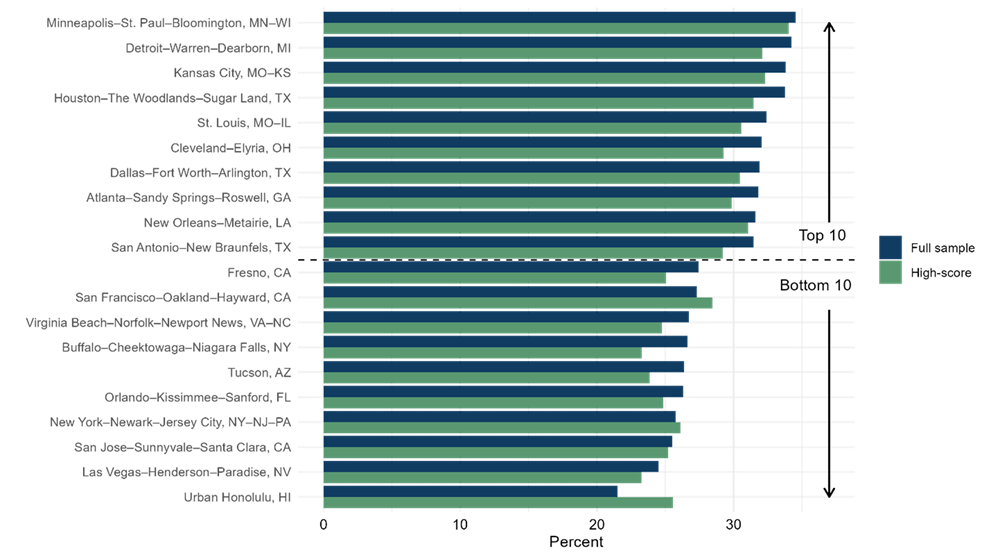
Sources: Federal Reserve Bank of New York/Equifax Consumer Credit Panel and authors’ calculations
The boomerang migration rate for people with high Equifax Risk Scores might be of particular interest because credit scores are positively correlated with income and education. As these people return, they are more likely to bring in-demand skills and purchasing power as consumers. We can see that, for most regions, the high-score boomerang rate is similar to the overall boomerang rate.
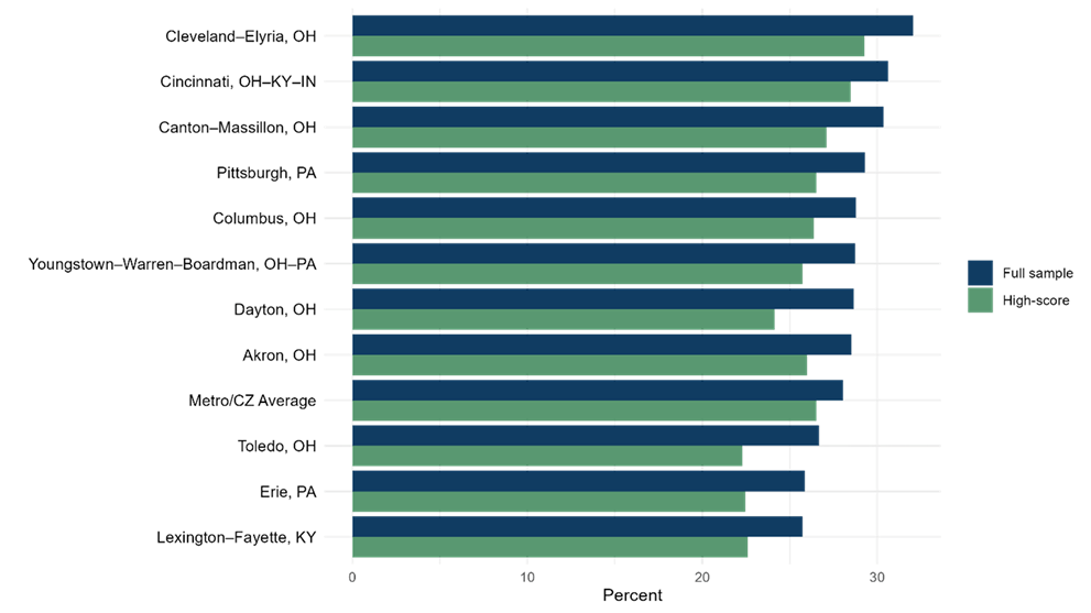
Across all metros and CZs, the population-weighted average boomerang rate is 28 percent. Figure 2 plots Fourth Federal Reserve District2 metros along with this average. On balance, the District’s metros perform well, with only Toledo, Erie, and Lexington attracting back fewer boomerang movers than the average region nationally. Although ranked last in the Fourth District by boomerang rate, Lexington has been among the District’s fastest-growing metros over the past two decades. Meanwhile, Cleveland, Canton, Pittsburgh, and Youngstown, each of which boast boomerang rates greater than the national average, have lower populations now than in 1999, the start of the study period. This begs the question of whether boomerang movers have a meaningful impact on the populations in their home regions.
Sources: Federal Reserve Bank of New York/Equifax Consumer Credit Panel and authors’ calculations
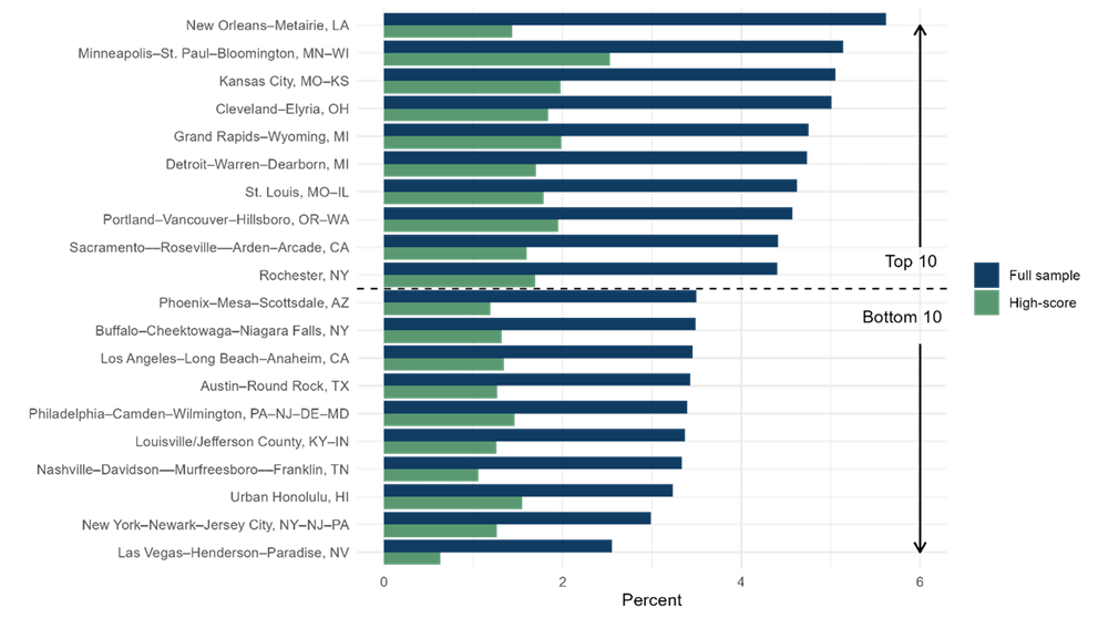
In Figure 3, we measure boomerang movers’ contribution to regional populations by taking the total number of quarters these movers spend at home after returning and dividing that figure by the total number of quarters we can observe for all individuals living in their home metro.3 While there is some variation between metros, the share of all quarters contributed by boomerang movers in any given region is limited, usually below 5 percent. The contributions from boomerang movers with top-third Equifax Risk Scores are under 2 percent because these are a subset (roughly one in three) of all boomerang movers. These modest levels mean that having a higher boomerang rate can provide only a small boost to a region’s population. For example, if a region with a boomerang share at the tenth percentile (3.7 percent) instead had a boomerang share equal to the ninetieth percentile (4.5 percent), its population level would have been only 0.8 percent higher during the study period.
Sources: Federal Reserve Bank of New York/Equifax Consumer Credit Panel and authors’ calculations
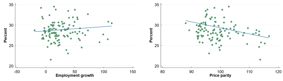
To increase boomerang migration via policy, one needs to know what motivates the migrants to return. Is it all about job growth? Does a low cost of living draw them back? In Figure 4, we plot regions’ boomerang rates over their job growth and a cost-of-living measure, the latter of which is an estimate from the Bureau of Economic Analysis of the prices in metro areas relative to national prices.4 We can see that employment growth from 1999 to 2023 is positively associated with the share of out-migrants that returned over those years. However, many regions with similar job growth have widely different boomerang rates. The relationship between the cost of living and boomerang migration appears more pronounced. In regions where prices averaged more than 5 percent above the national level (price parity >105), less than 30 percent of out-migrants return. Among regions with below-average prices (<100), there is wide variation: from 25 to 35 percent.
Sources: Federal Reserve Bank of New York/Equifax Consumer Credit Panel, Bureau of Economic Analysis, and authors’ calculations
Conclusion
Boomerang migration is very salient for residents and policymakers who remain in their home region because each likely has friends and relatives who have moved away. Knowing that many people returned after some time away gives hope that more natives will return to bolster the local population and economy. From this analysis, we learned that boomerang migration brings back 25 to 30 percent of most regions’ out-migrants, including people with healthy finances as indicated by their Equifax Risk Scores. However, because boomerang migrants account for only a small portion of a given region’s residents, even a relatively high rate of return among these migrants has a limited impact on the overall population level. For example, a rate of return of 33 percent instead of 25 percent would set a given region’s population level only about 1.5 percent higher.
The draw of being near family and friends is something regions cannot create for non-natives, but it usually already exists for people who grew up in the region. If resources are scarce for investing in amenities that will attract migrants, it is possible that reaching out to potential boomerang migrants is the least expensive opportunity to add to regional population growth. Strong regional job growth appears to be helpful to return migration but not a definitive driver of it. Moreover, although low prices in a region do not guarantee a high boomerang rate, very high prices seem to preclude one.
Footnotes
- Some students might use a college dormitory address in their first application for credit. If they are attending school out of town, they may be labeled natives of the wrong region. This could bias the estimates of retention, especially for college towns, because these students are likely to return home or move on after graduation. To account for this, we estimate the relationship between regions’ student populations and their retention. We then adjust each region’s retention estimate to remove the effect of students. Return to 1
- The Fourth District of the Federal Reserve System comprises Ohio, western Pennsylvania, eastern Kentucky, and the northern panhandle of West Virginia. Return to 2
- Because boomerang migrants can be identified only among people born after 1980, the total number of quarters for all the individuals in each region is also based on people born after 1980. Return to 3
- The regional price parities are available from 2008 through 2022. We use an average of the available years. Return to 4
Appendix
Table A1. Percent of Regions’ Native Out-Migrants That Return (Population >500,000)
| Boomerang rate | Boomerang rate | ||||
| Metro area | Full sample | High-score | Metro area | Full sample | High-score |
| Minneapolis–St. Paul–Bloomington, MN–WI | 34.5 | 34.0 | Charlotte–Concord–Gastonia, NC–SC | 28.4 | 25.4 |
| Detroit–Warren–Dearborn, MI | 34.2 | 32.1 | Riverside–San Bernardino–Ontario, CA | 28.3 | 26.4 |
| Kansas City, MO–KS | 33.8 | 32.3 | Bakersfield, CA | 28.2 | 24.6 |
| Houston–The Woodlands–Sugar Land, TX | 33.8 | 31.5 | Little Rock–North Little Rock–Conway, AR | 28.2 | 27.0 |
| Des Moines–West Des Moines, IA | 33.5 | 32.2 | Knoxville, TN | 28.1 | 26.6 |
| Boise City, ID | 32.7 | 32.1 | Milwaukee–Waukesha–West Allis, WI | 28.1 | 28.0 |
| St. Louis, MO–IL | 32.4 | 30.6 | Boston–Cambridge–Newton, MA–NH | 28.1 | 27.0 |
| Cleveland–Elyria, OH | 32.0 | 29.3 | Hartford–West Hartford–East Hartford, CT | 28.1 | 25.7 |
| Ogden–Clearfield, UT | 31.9 | 32.1 | Los Angeles–Long Beach–Anaheim, CA | 28.0 | 28.5 |
| Dallas–Fort Worth–Arlington, TX | 31.9 | 30.5 | Deltona–Daytona Beach–Ormond Beach, FL | 28.0 | 26.0 |
| Atlanta–Sandy Springs–Roswell, GA | 31.8 | 29.9 | Palm Bay–Melbourne–Titusville, FL | 28.0 | 24.3 |
| New Orleans–Metairie, LA | 31.6 | 31.1 | Baltimore–Columbia–Towson, MD | 28.0 | 26.1 |
| San Antonio–New Braunfels, TX | 31.5 | 29.2 | Nashville–Davidson–Murfreesboro–Franklin, TN | 27.9 | 25.4 |
| Provo–Orem, UT | 30.8 | 31.2 | Oxnard–Thousand Oaks–Ventura, CA | 27.8 | 27.8 |
| Portland–Vancouver–Hillsboro, OR–WA | 30.8 | 30.1 | Austin–Round Rock, TX | 27.7 | 26.0 |
| Jacksonville, FL | 30.8 | 26.9 | San Diego–Carlsbad, CA | 27.6 | 28.3 |
| Omaha–Council Bluffs, NE–IA | 30.6 | 29.8 | Rochester, NY | 27.6 | 24.6 |
| Portland–South Portland, ME | 30.6 | 30.5 | Lakeland–Winter Haven, FL | 27.5 | 26.6 |
| Cincinnati, OH–KY–IN | 30.6 | 28.5 | Miami–Fort Lauderdale–West Palm Beach, FL | 27.5 | 26.4 |
| McAllen–Edinburg–Mission, TX | 30.5 | 26.1 | Columbia, SC | 27.5 | 24.0 |
| Oklahoma City, OK | 30.4 | 28.2 | Fresno, CA | 27.4 | 25.1 |
| Indianapolis–Carmel–Anderson, IN | 30.3 | 28.6 | Greensboro–High Point, NC | 27.4 | 24.9 |
| Birmingham–Hoover, AL | 30.1 | 27.7 | Scranton–Wilkes–Barre–Hazleton, PA | 27.4 | 26.3 |
| Denver–Aurora–Lakewood, CO | 30.0 | 31.8 | Augusta–Richmond County, GA–SC | 27.3 | 23.7 |
| Grand Rapids–Wyoming, MI | 30.0 | 29.1 | San Francisco–Oakland–Hayward, CA | 27.3 | 28.4 |
| Winston–Salem, NC | 30.0 | 23.0 | Worcester, MA–CT | 27.3 | 24.7 |
| Spokane–Spokane Valley, WA | 29.9 | 29.4 | North Port–Sarasota–Bradenton, FL | 27.2 | 25.9 |
| Salt Lake City, UT | 29.8 | 29.2 | Baton Rouge, LA | 27.2 | 22.3 |
| Greenville–Anderson–Mauldin, SC | 29.8 | 26.2 | Wichita, KS | 27.0 | 25.2 |
| Tulsa, OK | 29.7 | 29.0 | Syracuse, NY | 26.9 | 23.2 |
| Sacramento–Roseville–Arden–Arcade, CA | 29.6 | 28.7 | Virginia Beach–Norfolk–Newport News, VA–NC | 26.7 | 24.8 |
| Memphis, TN–MS–AR | 29.6 | 23.2 | Stockton–Lodi, CA | 26.7 | 26.2 |
| Pittsburgh, PA | 29.3 | 26.5 | Charleston–North Charleston, SC | 26.7 | 24.5 |
| Seattle–Tacoma–Bellevue, WA | 29.3 | 29.0 | Toledo, OH | 26.7 | 22.3 |
| Phoenix–Mesa–Scottsdale, AZ | 29.2 | 28.2 | Buffalo–Cheektowaga–Niagara Falls, NY | 26.6 | 23.3 |
| Philadelphia–Camden–Wilmington, PA–NJ–DE–MD | 29.2 | 28.7 | Cape Coral–Fort Myers, FL | 26.5 | 23.9 |
| Providence–Warwick, RI–MA | 29.1 | 28.0 | Tucson, AZ | 26.4 | 23.8 |
| El Paso, TX | 29.0 | 27.7 | Orlando–Kissimmee–Sanford, FL | 26.3 | 24.8 |
| Louisville/Jefferson County, KY–IN | 29.0 | 28.9 | Albuquerque, NM | 26.2 | 23.6 |
| Chattanooga, TN–GA | 29.0 | 27.3 | Springfield, MA | 26.2 | 23.9 |
| Richmond, VA | 29.0 | 28.4 | Fayetteville–Springdale–Rogers, AR–MO | 25.8 | 25.2 |
| Chicago–Naperville–Elgin, IL–IN–WI | 28.9 | 27.4 | New York–Newark–Jersey City, NY–NJ–PA | 25.7 | 26.1 |
| Tampa–St. Petersburg–Clearwater, FL | 28.9 | 27.8 | Lexington–Fayette, KY | 25.7 | 22.6 |
| Harrisburg–Carlisle, PA | 28.8 | 26.1 | Lancaster, PA | 25.5 | 22.6 |
| Columbus, OH | 28.8 | 26.4 | San Jose–Sunnyvale–Santa Clara, CA | 25.5 | 25.2 |
| Washington–Arlington–Alexandria, DC–VA–MD–WV | 28.8 | 27.2 | New Haven–Milford, CT | 25.4 | 23.2 |
| Youngstown–Warren–Boardman, OH–PA | 28.7 | 25.7 | Madison, WI | 25.2 | 23.3 |
| Raleigh, NC | 28.7 | 28.2 | Allentown–Bethlehem–Easton, PA–NJ | 25.0 | 26.3 |
| Dayton, OH | 28.7 | 24.1 | Bridgeport–Stamford–Norwalk, CT | 24.6 | 24.4 |
| Modesto, CA | 28.6 | 26.8 | Las Vegas–Henderson–Paradise, NV | 24.5 | 23.2 |
| Akron, OH | 28.5 | 26.0 | Colorado Springs, CO | 23.9 | 22.6 |
| Albany–Schenectady–Troy, NY | 28.5 | 26.1 | Durham–Chapel Hill, NC | 23.1 | 20.2 |
| Jackson, MS | 28.4 | 26.1 | Urban Honolulu, HI | 21.5 | 25.6 |
Sources: Federal Reserve Bank of New York/Equifax Consumer Credit Panel and authors’ calculations
Table A2. Percent of All Observed Quarters Contributed by Returned Migrants (Population >500,000)
| Boomerang share | Boomerang share | ||||
| Metro area | Full sample | High-score | Metro area | Full sample | High-score |
| New Orleans–Metairie, LA | 5.6 | 1.4 | Richmond, VA | 4.0 | 1.5 |
| Provo–Orem, UT | 5.6 | 2.8 | Stockton–Lodi, CA | 4.0 | 1.2 |
| Des Moines–West Des Moines, IA | 5.4 | 2.3 | Little Rock–North Little Rock–Conway, AR | 4.0 | 1.2 |
| Minneapolis–St. Paul–Bloomington, MN–WI | 5.1 | 2.5 | Oklahoma City, OK | 4.0 | 1.2 |
| Kansas City, MO–KS | 5.1 | 2.0 | San Antonio–New Braunfels, TX | 4.0 | 1.0 |
| Boise City, ID | 5.0 | 2.0 | Columbia, SC | 3.9 | 0.9 |
| Cleveland–Elyria, OH | 5.0 | 1.8 | Jacksonville, FL | 3.9 | 0.9 |
| Portland–South Portland, ME | 4.8 | 1.9 | Toledo, OH | 3.9 | 1.2 |
| Grand Rapids–Wyoming, MI | 4.8 | 2.0 | Virginia Beach–Norfolk–Newport News, VA–NC | 3.9 | 1.0 |
| Detroit–Warren–Dearborn, MI | 4.7 | 1.7 | Tampa–St. Petersburg–Clearwater, FL | 3.9 | 1.0 |
| Ogden–Clearfield, UT | 4.7 | 2.5 | Miami–Fort Lauderdale–West Palm Beach, FL | 3.9 | 1.0 |
| St. Louis, MO–IL | 4.6 | 1.8 | San Diego–Carlsbad, CA | 3.9 | 1.5 |
| Portland–Vancouver–Hillsboro, OR–WA | 4.6 | 2.0 | Birmingham–Hoover, AL | 3.9 | 1.2 |
| Winston–Salem, NC | 4.6 | 1.1 | Dallas–Fort Worth–Arlington, TX | 3.9 | 1.3 |
| Palm Bay–Melbourne–Titusville, FL | 4.5 | 1.2 | Pittsburgh, PA | 3.9 | 1.7 |
| Oxnard–Thousand Oaks–Ventura, CA | 4.5 | 1.9 | Boston–Cambridge–Newton, MA–NH | 3.9 | 1.8 |
| Spokane–Spokane Valley, WA | 4.5 | 1.7 | Lakeland–Winter Haven, FL | 3.9 | 0.7 |
| Dayton, OH | 4.5 | 1.3 | New Haven–Milford, CT | 3.9 | 1.3 |
| Syracuse, NY | 4.5 | 1.6 | Jackson, MS | 3.9 | 0.9 |
| Harrisburg–Carlisle, PA | 4.5 | 1.7 | Chattanooga, TN–GA | 3.9 | 1.1 |
| Worcester, MA–CT | 4.5 | 1.6 | Scranton–Wilkes–Barre–Hazleton, PA | 3.8 | 1.4 |
| Akron, OH | 4.4 | 1.5 | Orlando–Kissimmee–Sanford, FL | 3.8 | 1.0 |
| Youngstown–Warren–Boardman, OH–PA | 4.4 | 1.4 | Durham–Chapel Hill, NC | 3.8 | 1.3 |
| Omaha–Council Bluffs, NE–IA | 4.4 | 1.9 | Riverside–San Bernardino–Ontario, CA | 3.8 | 1.0 |
| Modesto, CA | 4.4 | 1.2 | Chicago–Naperville–Elgin, IL–IN–WI | 3.8 | 1.6 |
| Sacramento–Roseville–Arden–Arcade, CA | 4.4 | 1.6 | Providence–Warwick, RI–MA | 3.8 | 1.4 |
| Rochester, NY | 4.4 | 1.7 | Baltimore–Columbia–Towson, MD | 3.8 | 1.4 |
| Albany–Schenectady–Troy, NY | 4.4 | 1.7 | Bakersfield, CA | 3.7 | 0.9 |
| Deltona–Daytona Beach–Ormond Beach, FL | 4.4 | 1.0 | Allentown–Bethlehem–Easton, PA–NJ | 3.7 | 1.6 |
| Tulsa, OK | 4.3 | 1.2 | Columbus, OH | 3.7 | 1.4 |
| Madison, WI | 4.3 | 2.2 | Memphis, TN–MS–AR | 3.7 | 0.7 |
| San Francisco–Oakland–Hayward, CA | 4.3 | 2.2 | Augusta–Richmond County, GA–SC | 3.7 | 0.6 |
| Springfield, MA | 4.3 | 1.3 | Charlotte–Concord–Gastonia, NC–SC | 3.6 | 1.1 |
| Washington–Arlington–Alexandria, DC–VA–MD–WV | 4.3 | 1.7 | Lexington–Fayette, KY | 3.6 | 1.2 |
| Salt Lake City, UT | 4.2 | 1.9 | Lancaster, PA | 3.6 | 1.5 |
| Raleigh, NC | 4.2 | 1.7 | Knoxville, TN | 3.6 | 1.3 |
| El Paso, TX | 4.2 | 0.8 | Baton Rouge, LA | 3.6 | 0.8 |
| Greensboro–High Point, NC | 4.2 | 1.1 | Tucson, AZ | 3.6 | 1.1 |
| North Port–Sarasota–Bradenton, FL | 4.2 | 1.2 | Fresno, CA | 3.5 | 0.9 |
| Wichita, KS | 4.2 | 1.6 | Phoenix–Mesa–Scottsdale, AZ | 3.5 | 1.2 |
| Hartford–West Hartford–East Hartford, CT | 4.2 | 1.7 | Buffalo–Cheektowaga–Niagara Falls, NY | 3.5 | 1.3 |
| Cincinnati, OH–KY–IN | 4.2 | 1.7 | McAllen–Edinburg–Mission, TX | 3.5 | 0.6 |
| Indianapolis–Carmel–Anderson, IN | 4.2 | 1.4 | Los Angeles–Long Beach–Anaheim, CA | 3.5 | 1.3 |
| Denver–Aurora–Lakewood, CO | 4.2 | 2.1 | Austin–Round Rock, TX | 3.4 | 1.3 |
| San Jose–Sunnyvale–Santa Clara, CA | 4.2 | 2.2 | Philadelphia–Camden–Wilmington, PA–NJ–DE–MD | 3.4 | 1.5 |
| Houston–The Woodlands–Sugar Land, TX | 4.2 | 1.4 | Louisville/Jefferson County, KY–IN | 3.4 | 1.3 |
| Colorado Springs, CO | 4.1 | 1.6 | Nashville–Davidson–Murfreesboro–Franklin, TN | 3.3 | 1.1 |
| Atlanta–Sandy Springs–Roswell, GA | 4.1 | 1.3 | Charleston–North Charleston, SC | 3.3 | 0.9 |
| Milwaukee–Waukesha–West Allis, WI | 4.1 | 1.9 | Albuquerque, NM | 3.3 | 1.0 |
| Bridgeport–Stamford–Norwalk, CT | 4.1 | 1.8 | Fayetteville–Springdale–Rogers, AR–MO | 3.3 | 1.1 |
| Seattle–Tacoma–Bellevue, WA | 4.0 | 1.9 | Urban Honolulu, HI | 3.2 | 1.6 |
| Greenville–Anderson–Mauldin, SC | 4.0 | 1.3 | New York–Newark–Jersey City, NY–NJ–PA | 3.0 | 1.3 |
| Cape Coral–Fort Myers, FL | 4.0 | 0.9 | Las Vegas–Henderson–Paradise, NV | 2.6 | 0.6 |
Sources: Federal Reserve Bank of New York/Equifax Consumer Credit Panel and authors’ calculations
Table A3. Boomerang Rate and Share (Population-Weighted Average, Population ≤500,000)
| Boomerang rate | Boomerang share | ||||
| Metro area | Full sample | High-score | Metro area | Full sample | High-score |
| Small metro and rural – Oregon | 27.9 | 26.8 | Small metro and rural – Minnesota | 5.7 | 2.3 |
| Small metro and rural – Ohio | 27.9 | 25.2 | Small metro and rural – Idaho | 5.6 | 2.0 |
| Small metro and rural – Alabama | 27.8 | 23.8 | Small metro and rural – Montana | 5.5 | 2.1 |
| Small metro and rural – Georgia | 27.5 | 23.4 | Small metro and rural – Iowa | 5.4 | 2.1 |
| Small metro and rural – Louisiana | 27.4 | 25.4 | Small metro and rural – South Dakota | 5.3 | 2.2 |
| Small metro and rural – Maine | 27.3 | 24.4 | Small metro and rural – North Dakota | 5.3 | 2.4 |
| Small metro and rural – Washington | 27.1 | 26.0 | Small metro and rural – Oregon | 5.3 | 1.7 |
| Small metro and rural – Idaho | 27.1 | 26.6 | Small metro and rural – Ohio | 5.3 | 1.5 |
| Small metro and rural – Maryland | 27.1 | 24.3 | Small metro and rural – Kansas | 5.2 | 1.9 |
| Small metro and rural – California | 27.1 | 27.2 | Small metro and rural – Wisconsin | 5.1 | 2.1 |
| Small metro and rural – Kentucky | 27.0 | 24.7 | Small metro and rural – Michigan | 5.1 | 1.6 |
| Small metro and rural – Montana | 26.8 | 27.0 | Small metro and rural – Nebraska | 5.1 | 2.1 |
| Small metro and rural – West Virginia | 26.8 | 23.8 | Small metro and rural – Missouri | 5.1 | 1.3 |
| Small metro and rural – New Hampshire | 26.8 | 23.8 | Small metro and rural – Washington | 4.9 | 1.7 |
| Small metro and rural – Michigan | 26.7 | 24.2 | Small metro and rural – Illinois | 4.9 | 1.7 |
| Small metro and rural – Mississippi | 26.6 | 23.4 | Small metro and rural – Indiana | 4.9 | 1.5 |
| Small metro and rural – New Jersey | 26.6 | 23.2 | Small metro and rural – Arizona | 4.8 | 1.2 |
| Small metro and rural – Tennessee | 26.6 | 23.9 | Small metro and rural – Utah | 4.8 | 2.2 |
| Small metro and rural – Texas | 26.5 | 23.1 | Small metro and rural – New Hampshire | 4.8 | 1.6 |
| Small metro and rural – Minnesota | 26.4 | 25.2 | Small metro and rural – California | 4.8 | 1.7 |
| Small metro and rural – Indiana | 26.3 | 23.3 | Small metro and rural – New York | 4.7 | 1.4 |
| Small metro and rural – Pennsylvania | 26.3 | 24.3 | Small metro and rural – Oklahoma | 4.6 | 0.9 |
| Small metro and rural – Wisconsin | 26.3 | 24.0 | Small metro and rural – Texas | 4.6 | 0.8 |
| Small metro and rural – New York | 26.3 | 23.5 | Small metro and rural – Maine | 4.6 | 1.4 |
| Small metro and rural – Delaware | 26.2 | 24.4 | Small metro and rural – Wyoming | 4.6 | 1.5 |
| Small metro and rural – Missouri | 26.1 | 23.6 | Small metro and rural – Pennsylvania | 4.5 | 1.6 |
| Small metro and rural – North Carolina | 26.0 | 23.1 | Small metro and rural – Colorado | 4.5 | 1.7 |
| Small metro and rural – Florida | 25.8 | 23.3 | Small metro and rural – Florida | 4.5 | 1.0 |
| Small metro and rural – Illinois | 25.6 | 23.3 | Small metro and rural – Georgia | 4.4 | 0.8 |
| Small metro and rural – Virginia | 25.6 | 23.3 | Small metro and rural – Mississippi | 4.4 | 0.7 |
| Small metro and rural – Vermont | 25.5 | 24.9 | Small metro and rural – Vermont | 4.4 | 1.8 |
| Small metro and rural – South Dakota | 25.4 | 24.8 | Small metro and rural – Alabama | 4.4 | 0.9 |
| Small metro and rural – North Dakota | 25.4 | 25.8 | Small metro and rural – Virginia | 4.4 | 1.2 |
| Small metro and rural – Massachusetts | 25.2 | 23.6 | Small metro and rural – Kentucky | 4.4 | 1.0 |
| Small metro and rural – Connecticut | 25.1 | 21.8 | Small metro and rural – Maryland | 4.4 | 1.2 |
| Small metro and rural – South Carolina | 25.1 | 22.1 | Small metro and rural – Tennessee | 4.4 | 1.0 |
| Small metro and rural – Nevada | 24.7 | 25.4 | Small metro and rural – Arkansas | 4.3 | 0.9 |
| Small metro and rural – Iowa | 24.7 | 23.5 | Small metro and rural – Connecticut | 4.2 | 1.6 |
| Small metro and rural – Oklahoma | 24.7 | 22.2 | Small metro and rural – Louisiana | 4.2 | 0.9 |
| Small metro and rural – Arkansas | 24.6 | 23.3 | Small metro and rural – Massachusetts | 4.2 | 1.6 |
| Small metro and rural – Arizona | 24.4 | 23.3 | Small metro and rural – New Mexico | 4.2 | 1.0 |
| Small metro and rural – Colorado | 24.2 | 23.9 | Small metro and rural – West Virginia | 4.2 | 0.9 |
| Small metro and rural – New Mexico | 23.9 | 22.0 | Small metro and rural – North Carolina | 4.1 | 0.9 |
| Small metro and rural – Nebraska | 23.8 | 23.2 | Small metro and rural – Nevada | 4.1 | 1.3 |
| Small metro and rural – Utah | 23.6 | 23.9 | Small metro and rural – New Jersey | 4.0 | 1.2 |
| Small metro and rural – Kansas | 23.5 | 22.4 | Small metro and rural – South Carolina | 3.9 | 0.6 |
| Small metro and rural – Hawaii | 23.3 | 25.7 | Small metro and rural – Hawaii | 3.9 | 1.7 |
| Small metro and rural – Wyoming | 22.7 | 21.2 | Small metro and rural – Delaware | 3.8 | 1.0 |
| Small metro and rural – Alaska | 21.8 | 22.3 | Small metro and rural – Alaska | 3.8 | 1.3 |
Notes: Boomerang rates are first calculated for each small metro and CZ and then combined via a population-weighted average. Individuals who move between small metros or CZs within the same state contribute to the rate calculation in the same way as people moving between major metros. Metros and CZs that cross state lines are assigned to the state with the highest share of their population.
Sources: Federal Reserve Bank of New York/Equifax Consumer Credit Panel and authors’ calculations
Suggested Citation
Whitaker, Stephan D., and Brett Huettner. 2025. “Boomerang Migration: Which Regions Have the Most, and Can It Make a Difference?” Federal Reserve Bank of Cleveland, Cleveland Fed District Data Brief. https://doi.org/10.26509/frbc-ddb-20250219
This work by Federal Reserve Bank of Cleveland is licensed under Creative Commons Attribution-NonCommercial 4.0 International


- Share

Regional Data, Analysis, and Engagement
Explore economic trends and the circumstances impacting the economy and diverse communities of the Federal Reserve’s Fourth District, which includes all of Ohio, western Pennsylvania, eastern Kentucky, and the northern panhandle of West Virginia.